Neural Network Can Learn Any Pattern

Posted Nov 17, 2023 Updated Feb 23, 2024

By tracywong 10 min read

Universal approximation theorem

To begin with, the most important thing to know is that neural networks can approximate anything that can be expressed as a function. It is stated by the Universal approximation theorem proved in 1989, which means that given a sufficient number of neurons and appropriate training, they can approximate any function to any degree of precision. That’s why neural network can learn complex, nonlinear relationships between inputs and outputs.

Note that inputs can be an image, a video, a text, an audio and any other kind of record that can be represented be number (or more concise: vector). For example, if we provide a neural network with an image of a dog, it can output a label indicating that it is indeed a dog. Similarly, in the case of converting speech to text, the neural network acts as a tool to accomplish this task. Neural networks transform inputs into desired outputs, just like traditional mathematical functions.

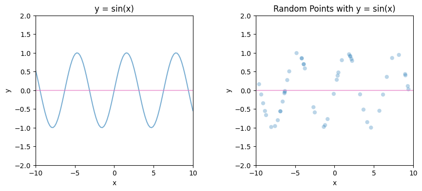
One way to view neural networks is as a form of reverse engineering. When you have a set of data generated by an unknown function, let’s say $y = sin(x)$, a neural network can learn to approximate this function without explicitly knowing its mathematical form. By training the network on the available data points, it can infer the underlying patterns. We will say the actual function $f(x)$ is approximate by neural network as another function $T(x)$.

\[f(x)=sin(x) \approx T(x)\]

Let’s work on actual example

Requirements:
Python3
PyTorch
Numpy
Sklearn
Matplotlib
It is strongly recommended to use Google Colab to run the code below. They provide free computation resource and have pre-installed most of the common machine learning library.

So, here is the randomly generated dataset. The points that are inside the circle is labeled as 0 (blue). The points that are outside the circle is labeled as 1 (orange). Note that the function of a circle is stated as

\[x^2 + y^2 = radius\]

Here, we put $radius = 1$.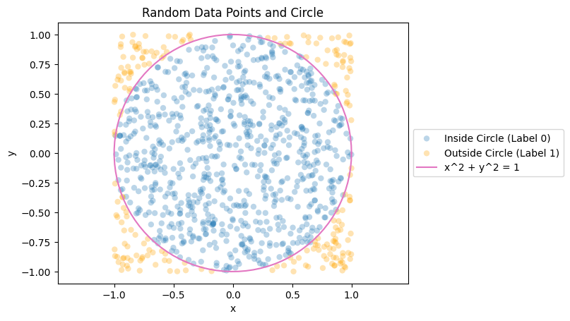

Our task is to approximate the function of the circle by letting neural network to learn from the data points.

Let’s think it step by step.

Architecture of a neural network

The architecture of a neural network is a key component. It may surprise you how few lines of code are needed to define a neural network.

  
class NeuralNetwork(nn.Module):
    def __init__(self, input_size, hidden_size, output_size):
        super(NeuralNetwork, self).__init__()
        self.fc1 = nn.Linear(input_size, hidden_size)
        self.fc2 = nn.Linear(hidden_size, output_size)
        self.relu = nn.ReLU()
        
    def forward(self, x):
        x = self.fc1(x)
        x = self.relu(x)
        x = self.fc2(x)
        x = self.relu(x)
        return x

fc1 and fc2 are referred to fully-connected layer while relu is referred to rectified linear unit (ReLU) used as activation function of fully connected layer. The neural network consists solely of fully connected layers and their activation functions.

A fully connected layer connects every neuron from previous layer (input) to every neuron in this layer (output). The fully connected layer is defned by batch size, number of inputs, and number of outputs. A ReLU is used to introduce non-linearity after each fully connected layer.

It can be expressed mathematically as:

For each output neuron, the resulting value will be a scalar.

\[\begin{align*} N(x_1, x_2, ..., x_n) &= w_1x_1 + w_2x_2 + ... + w_nx_n + bias \\ &= wx + bias \end{align*}\] \[w = \begin{bmatrix} w_1 & w_2 & ... & w_n \end{bmatrix}\] \[x= \begin{bmatrix} x_1 \\ x_2 \\ ... \\ x_n \end{bmatrix}\]

For the entire fully connected layer, the resulting matrix will have dimensions of $m\times1$ where $m$ is the number of outputs.

\[FC(X) = Wx + b\] \[W = \begin{bmatrix} w_{1,1} & w_{2,1} & ... & w_{n,1} \\ w_{1,2} & w_{2,2} & ... & w_{n,2} \\ ... & ... & ... & ... \\ w_{1,m} & w_{2,m} & ... & w_{n,m} \end{bmatrix}\] \[b= \begin{bmatrix} b_1 \\ b_2 \\ ... \\ b_m \end{bmatrix}\]

For the activation function ReLU,

\[ReLU(x) = MAX(x, 0)\]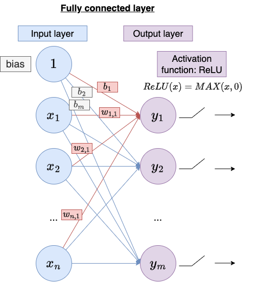

The parameters of our neural network are as follows:

  
# Define the hyperparameters
input_size = 2
hidden_size = 4
output_size = 1
learning_rate = 0.1
num_epochs = 2000

# Create the neural network
model = NeuralNetwork(input_size, hidden_size, output_size)

Feel free to try different parameters.

Training process

  
# Define the loss function and optimizer
criterion = nn.MSELoss()
optimizer = optim.SGD(model.parameters(), lr=learning_rate)

history = []

# Training loop
for epoch in range(num_epochs):
    # Forward pass
    outputs = model(X_train_tensor)
    loss = criterion(outputs, y_train_tensor)
    
    # Backward and optimize
    optimizer.zero_grad()
    loss.backward()
    optimizer.step()

    history.append(loss.item())
    
    # Print the loss for every 100 epochs
    if epoch % 100 == 0:
        print(f"Epoch {epoch}: Loss = {loss.item():.4f}")

torch.nn.MSELoss
Creates a criterion that measures the mean squared error (squared L2 norm) between each element in the input x and target y.

MSE (Mean Squared Error)

\[MSE = \frac{1}{n} \sum_{i=1}^{n}(Y_i - \hat{Y}_i)^2\]

where $n$ is the number of data points, $Y_i$ is the observed value (target) and $\hat{Y}_i$ is the predicted value (input).

Backpropagation

Backpropagation is a technique used in training neural networks to adjust the parameters (weights and biases) of the network based on the computed loss. The primary goal of backpropagation is to minimize the difference between the predicted output of the neural network and the desired output, which is measured by the loss function. In this sense, backpropagation serves as the key mechanism by which neural networks learn from data.

torch.optim.Optimizer.zero_grad
Resets the gradients of all optimized parameters.
Gradients are accumulated. Before calculating the gradients for a new batch of data, it’s necessary to zero them out.

torch.Tensor.backward
Performs backward propagation of the loss between input and output. It calculates gradients $\frac{d}{dx} loss$ for all variables that require gradient computation (i.e., have requires_grad=True), and accumulates them in the gradient tensor (grad): $x.grad = x.grad + \frac{d}{dx} loss$
The graph is differentiated using the chain rule.

torch.optim.Optimizer.step
Updates the values of the variables using the optimizer. Taking stochastic gradient descent (SGD) as an example, it adjusts the variable values by subtracting the product of the learning rate (lr) and the gradient. $x=x-lr*x.grad$

Try out torch.Tensor.backward

Let’s use a simple function to observe the behavior of torch.Tensor.backward.

  
x = torch.tensor(np.array([-10.0, 5.0]), requires_grad=True)
print(x)
# tensor([-10.,   5.], dtype=torch.float64, requires_grad=True)
print(x.grad)
# None

torch.sum(x**2).backward()
print(x.grad)
# tensor([-20.,  10.], dtype=torch.float64)

torch.sum(x**2).backward()
=> $f = a^2 + b^2$ where $a = -10.0$ and $b = 5.0$ in this case
\[\frac{df}{da} = \frac{d(a^2+b^2)}{da} = 2a\]
$x.grad[0] = x.grad + \frac{df}{da} = 0 + 2a = -20$
$x.grad[1] = x.grad + \frac{df}{db} = 0 + 2b = 10$

Do this again

  
# without x.zero_grad(), x.grad is accumulating
torch.sum(x**2).backward()
print(x.grad)
# tensor([-40.,  20.], dtype=torch.float64)

$x.grad[0] = x.grad + \frac{df}{da} = -20 + 2a = -40$
$x.grad[1] = x.grad + \frac{df}{db} = 10 + 2b = 20$

When calling backward() on a tensor, the gradients are calculated and accumulated in the grad attribute of the tensor. If multiple backward passes are performed without resetting the gradients using zero_grad(), the gradients are accumulated across those passes.

Result

Visualization of prediction

The training result is as follows: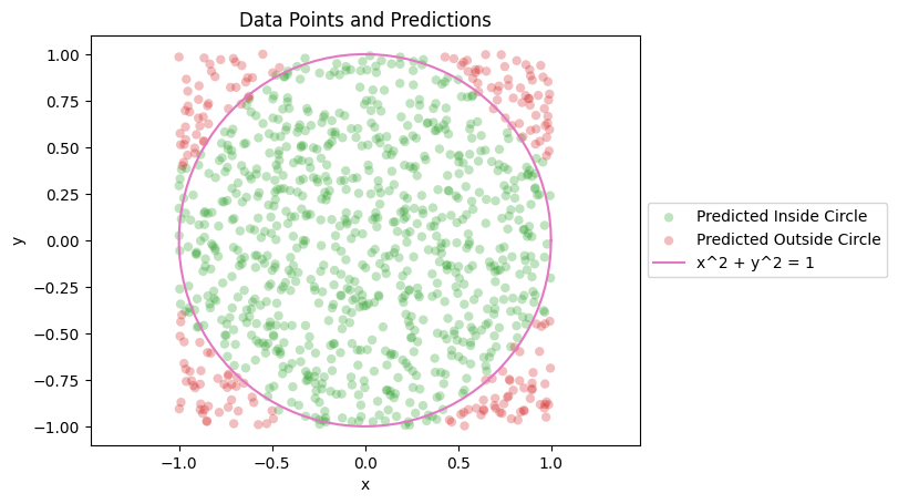

We observe that the majority of predictions are accurate. Most of the green data points fall within the circle, aligning with the expected outcome. Likewise, nearly all red data points lie outside the circle.

Accuracy

Test Loss: 0.0423
Accuracy: 96.00%

Training loss

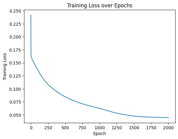
The training loss consistently decreases as the model progresses through each epoch.

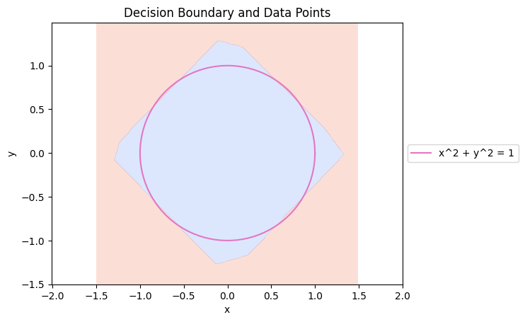
Decision boundary

Below is the decision boundary indicating the neural network’s predictions, with the orange area representing predictions labeled as 1 (data point outside the circle) and the purple area representing predictions labeled as 0 (data point inside the circle).

Code

Training and Evaluating

  
import torch
import torch.nn as nn
import torch.optim as optim
from sklearn.model_selection import train_test_split
import numpy as np
import matplotlib.pyplot as plt

class NeuralNetwork(nn.Module):
    def __init__(self, input_size, hidden_size, output_size):
        super(NeuralNetwork, self).__init__()
        self.fc1 = nn.Linear(input_size, hidden_size)
        self.fc2 = nn.Linear(hidden_size, output_size)
        self.relu = nn.ReLU()
        
    def forward(self, x):
        x = self.fc1(x)
        x = self.relu(x)
        x = self.fc2(x)
        x = self.relu(x)
        return x

# Generate random x and y coordinates
num_points = 10000
x = np.random.uniform(low=-1, high=1, size=num_points)
y = np.random.uniform(low=-1, high=1, size=num_points)

# Assign labels based on whether points fall inside or outside the circle
labels = np.where(x**2 + y**2 <= 1, 0, 1)

# Combine the coordinates into input data
X = np.column_stack((x, y))

# Split the data into training and testing datasets
X_train, X_test, y_train, y_test = train_test_split(X, labels, test_size=0.1, random_state=42)

# Convert data to PyTorch tensors
X_train_tensor = torch.tensor(X_train, dtype=torch.float32)
y_train_tensor = torch.tensor(y_train, dtype=torch.float32).unsqueeze(1)
X_test_tensor = torch.tensor(X_test, dtype=torch.float32)
y_test_tensor = torch.tensor(y_test, dtype=torch.float32).unsqueeze(1)

# Define the hyperparameters
input_size = 2
hidden_size = 4
output_size = 1
learning_rate = 0.1
num_epochs = 2000

# Create the neural network
model = NeuralNetwork(input_size, hidden_size, output_size)

# Define the loss function and optimizer
criterion = nn.MSELoss()
optimizer = optim.SGD(model.parameters(), lr=learning_rate)

history = []

# Training loop
for epoch in range(num_epochs):
    # Forward pass
    outputs = model(X_train_tensor)
    loss = criterion(outputs, y_train_tensor)
    
    # Backward and optimize
    optimizer.zero_grad()
    loss.backward()
    optimizer.step()

    history.append(loss.item())
    
    # Print the loss for every 100 epochs
    if epoch % 100 == 0:
        print(f"Epoch {epoch}: Loss = {loss.item():.4f}")

# Evaluation on the testing dataset
with torch.no_grad():
    model.eval()
    test_outputs = model(X_test_tensor)
    print(X_test_tensor, y_test_tensor)
    print(test_outputs)
    test_loss = criterion(test_outputs, y_test_tensor)
    predicted_labels = (test_outputs >= 0.5).squeeze().numpy()
    accuracy = np.mean(predicted_labels == y_test)

print(f"Test Loss: {test_loss.item():.4f}")
print(f"Accuracy: {accuracy * 100:.2f}%")

Plot graph

↓ Plotting this

  
# Plot the data points and predictions
plt.scatter(X_test[predicted_labels<0.5, 0], X_test[predicted_labels<0.5, 1], color='tab:green', alpha=0.3, edgecolors='none', label='Predicted Inside Circle')
plt.scatter(X_test[predicted_labels>=0.5, 0], X_test[predicted_labels>=0.5, 1], color='tab:red', alpha=0.3, edgecolors='none', label='Predicted Outside Circle')

# Plot the line x^2 + y^2 = 1
theta = np.linspace(0, 2*np.pi, 100)
x_circle = np.cos(theta)
y_circle = np.sin(theta)
plt.plot(x_circle, y_circle, color='tab:pink', label='x^2 + y^2 = 1')

plt.xlabel('x')
plt.ylabel('y')
plt.title('Data Points and Predictions')
plt.legend(loc='center left', bbox_to_anchor=(1, 0.5))
plt.axis('equal')
plt.show()